


 广告
广告


基于KKT原理和五次多项式的换道策略

车道换道行为是日常行车中最常见的驾驶行为之一,车辆换道轨迹规划是自主车辆能否安全而又高效地完成换道任务的关键,因此对换道轨迹规划的研究逐渐成为自主车辆技术研究的重点。基于几何的轨迹规划通常采用参数化的曲线来描述轨迹,这种方法较为直观、精确,且运算量较小,因此是目前采用的较为广泛的轨迹规划方法。本文根据换道过程中对换道轨迹平稳性、舒适性和效率性的要求,提出了一种基于五次多项式的换道轨迹规划方法。
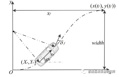
图1 车辆换道过程
假设车辆横纵向位置y(t)、x(t)是关于时间t的五次多项式:
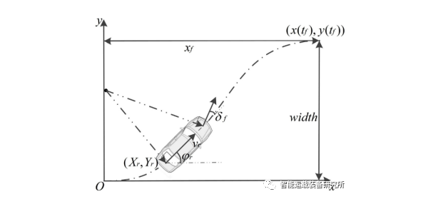
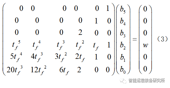
车辆换道轨迹规划实际上是求解式(1)中的系数ai和bi的值,基于多项式的换道轨迹模型只需获取车辆的初始状态及目标状态,即可通过计算获得换道轨迹,即建立边界条件
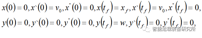
其中,w是车道宽度,tf和xf是完成整个换道过程所需的时间以及纵向行驶距离,v0表示换道时的纵向车速。
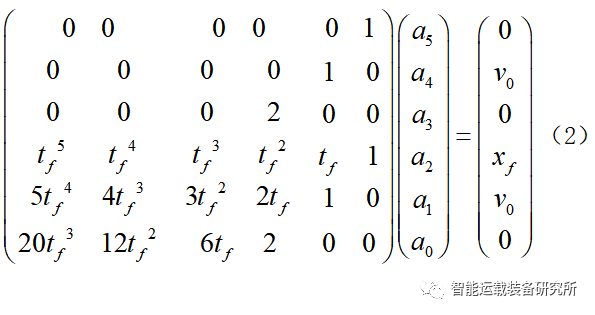
根据上述边界条件可得x和y关于t的六元一次方程组:
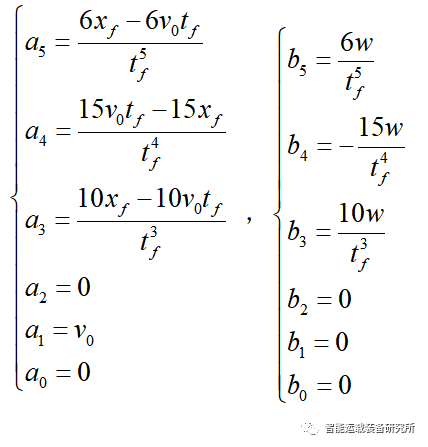
可得五次多项式的系数为:
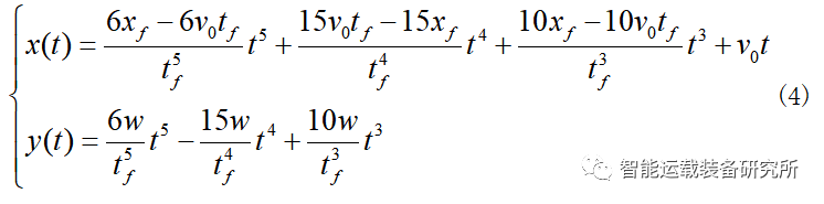
则可得换道轨迹的五次多项式为:
根据变道过程中对换道轨迹平稳性和效率性,以及变道效率的要求,所以对横纵向加速度以及变道纵向距离进行优化。换道轨迹规划时的代价函数为:
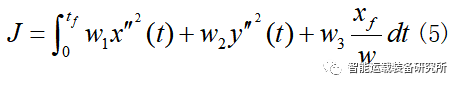
其中,w1,w2,w3分别是权重系数。
将换道轨迹方程代入优化目标函数可得:
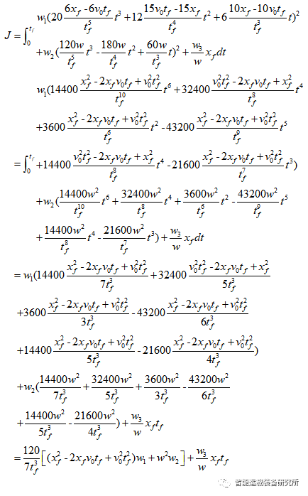
该优化目标是纵向行驶距离xf和换道时间tf的二元函数,根据KKT原理求解该优化函数的极值点:
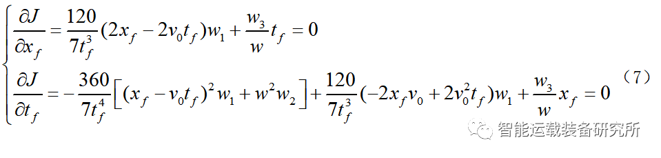
解该方程组可得最优解满足关系式:
考虑到横向的安全性与舒适性更重要,因此,选取权重系数为w1=w3=1,w2=2,道路宽度为w=3.5,MATLAB求解程序如下:
__________________________________________________________________________
clear,clc
w=3.5;w2=2;v0=linspace(5,50);
tf=zeros(1,length(v0));xf=zeros(1,length(v0));
for i=1:length(v0)
p=[49,0,0,-1344*w*v0(i),0,0,0,0,34560*w2*w^4];
t0=roots(p);
index=find(abs(imag(t0))<=1e-10&real(t0)>0);
tf(i)=min(t0(index));
xf(i)=v0(i)*tf(i)-7*tf(i)^4/240/w;
end
plot(tf,xf./v0);hold on;plot(tf,tf,'r');grid on
figure
plot(v0,tf)
figure
plot(v0,xf)
figure
plot(v0,xf-v0.*tf)
__________________________________________________________________________
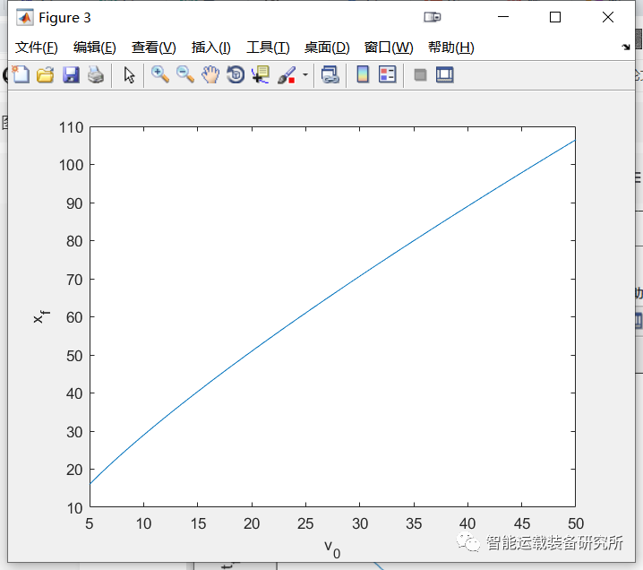
xf和tf与车速v0之间的关系如下图所示。可见,随着车速增大,tf逐渐减小并趋于稳定值,xf逐渐增大并趋于线性关系。在低速时为了保证安全,换道时间较大;在高速时为了追求换道效率,换道时间较小。通过仿真还可以发现,增大权重系数w2时,tf会增大,这是因为横向加速度的权重增大后换道过程更平缓了。
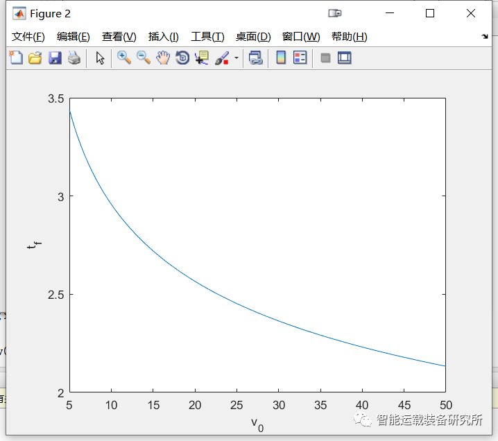
图2 换道时间与车速间的关系
图3 换道距离与车速间的关系
定义距离偏差e=xf-v0*tf,该误差与车速间的关系如下图所示,可见,随着车速的增大偏差逐渐减小,说明换道距离与换道时间之间的关系可以用线性来表示。因此,在换道决策以及路径规划时,可以选择如下的策略。
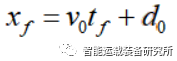
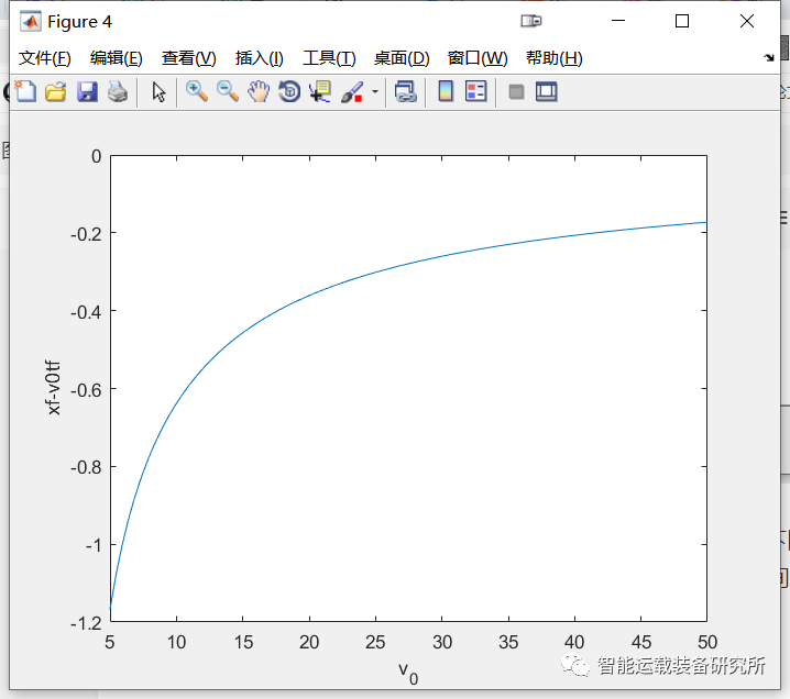
图4 换道距离偏差
图5 换道时间


编辑推荐


最新资讯
-
中汽中心工程院能量流测试设备上线全新专家
2025-04-03 08:46
-
上新|AutoHawk Extreme 横空出世-新一代实
2025-04-03 08:42
-
「智能座椅」东风日产N7为何敢称“百万级大
2025-04-03 08:31
-
基于加速度计补偿的俯仰角和路面坡度角估计
2025-04-03 08:30
-
《北京市自动驾驶汽车条例》正式实施 L3级
2025-04-02 20:23
